Introduction

The Spin Sampler library is designed to study the thermodynamical properties of spin glasses. It provides tools to sample from the Boltzmann distribution of a spin system using Gibbs sampling. This document explains the physical details, sampling procedure, and the algorithm used.

Physical Details

We consider a system of \(N\) binary spins \(\boldsymbol{s} = (s_1, \cdots, s_N) \in \{-1, +1\}^N\) coupled with the Hamiltonian:

\[H(\boldsymbol{s}) = -\frac{1}{2} \sum_{i=1}^N J_{ij} s_i s_j\]

where the coupling matrix \(\boldsymbol{J} = (J_{ij})\) is typically random. The system is assumed to be in equilibrium with a thermal bath at temperature \(T = 1 / \beta\), and the equilibrium configurations \(\boldsymbol{s}\) follow the Boltzmann distribution.

\[\mu(\boldsymbol{s}) = \frac{e^{-\beta H(\boldsymbol{s})}}{Z_\beta}.\]

To describe these systems, we rely on order parameters (e.g., \(q\)) that are averages over the Boltzmann measure, but in practice we aproximate them with a Monte Carlo estimate based on a number of samples \(N_S\).

\[q = \langle Q(\boldsymbol{s}) \rangle \equiv \sum_{\boldsymbol{s}} Q(\boldsymbol{s}) \mu(\boldsymbol{s}) \approx \frac{1}{N_S} \sum_{t=1}^{N_S} Q(\boldsymbol{s}^{(t)}).\]

Sampling Procedure

To sample from the Boltzmann distribution, we use Gibbs sampling. The algorithm updates spins one at a time using their conditional probability:

\[P(s_i = +1 \mid \boldsymbol{s}_{\setminus i}) = \frac{1}{1 + \exp(-2\beta h_i)},\]

where the local field at site \(i\) is given by

\[h_i = \sum_{j \neq i} J_{ij} s_j.\]

Algorithm

The Gibbs sampling algorithm starts at \(t=0\) with the initial configuration \(\boldsymbol{s}^{(0)} \in \{-1, +1\}^N, \;\) and continues as:

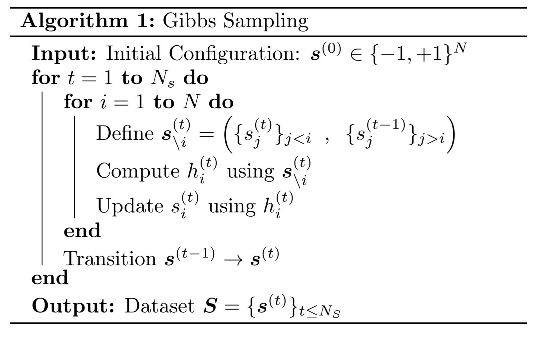
The only important thing to notice about the algorithm is that the inner loop over \(N\) (refered in the library as gibbs_step) must be done sequentially because the value of spin \(i\) at time \(t\) depends on the values of all other spins \(j<i\) that were already updated in the same \(t\). This is different from other sampling problems where the update \((t-1) \rightarrow(t)\) can be done in a single step and even if there are many variables involved one could use parallelization techniques to make the update efficient.